Cross Spectral Analysis Tutorial
This tutorial covers the spectral analysis capabilities of FlexPro when two signals need to be compared for spectral content. The Cross Spectrum, Cross Periodogram, and Coherence functions offer the means to evaluate similarity and dissimilarity between two signals. These procedures are often used for signals that come from the same source. But this does not have to be the case. Any two signals that have the same data length can be evaluated.
This tutorial also covers Fourier transfer functions between an input and output signal.
Fourier Analysis
If you have not already done so, it is recommended that you go through the Fourier Analysis tutorial before beginning this one. Most of the principles of Fourier analysis are covered in that tutorial. In this tutorial, we will highlight only the key items that occur when two separate signals are evaluated using cross-Fourier spectral methods.
Two Test Signals
For this tutorial, we will use two 1024 length signals. The first will be a reference signal containing nine equal power sinusoids spaced evenly across the Nyquist range:
100.0*sin(2π*x*250+p)
100.0*sin(2π*x*500+p)
100.0*sin(2π*x*750+p)
100.0*sin(2π*x*1000+p)
100.0*sin(2π*x*1250+p)
100.0*sin(2π*x*1500+p)
100.0*sin(2π*x*1750+p)
100.0*sin(2π*x*2000+p)
100.0*sin(2π*x*2250+p)
To see the impact of varying amplitudes, frequencies, and phases in a cross-spectral analysis, we modified the components in the second signal as follows:
100.0*sin(2π*x*250+p)
75.0*sin(2π*x*500+p)
50.0*sin(2π*x*750+p)
25.0*sin(2π*x*1000+p)
0.0*sin(2π*x*1250+p)
100.0*sin(2π*x*1502.5+p)
100.0*sin(2π*x*1775+p)
100.0*sin(2π*x*2000+0)
100.0*sin(2π*x*2250+p/2)
The first five components have a linear decay from 100% to 0% amplitude. The next two components shift upward in frequency 0.1% and 1% of the Nyquist range. The last two components have a -p and -p/2 phase shift.
The sampling rate is 5000 Hz. Thus, the Nyquist frequency is 2500 Hz, the maximum frequency that can be detected. The time values vary from 0 to 0.2046 at a 0.0002 sample increment. 10% random Gaussian noise was added to both signals. This produces a noise floor at about -40 dB relative to the largest peak.
Select the command File > Open Project Database and open the project database C:\Users\Public\Documents\Weisang\FlexPro\2021\Examples\Tutorials\Spectral Analysis.fpd or C:>Users>Public>Public Documents>Weisang>FlexPro>2021>Examples\Tutorials\Spectral Analysis.fpd. Open the Tutorials folder and its Cross Spectral Analysis subfolder and then double-click to open the 2D diagram called Data.
This is a graph of both signals. There are 1024 floating point values.
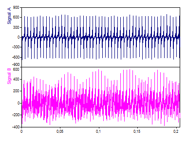
From the time-domain, about all that can be inferred is that there are significant similarities as well as significant differences.
Fourier Spectra
Close the diagram and highlight the data set Signal A, the reference signal.
Click on Insert[Analyses] > Analysis Wizard.
Select the Spectral Analyses category and then Fourier Analyses. Next, select Fourier Spectrum. Note that the result of some spectral procedures depends on the order of the selected data sets. You should therefore always carefully verify that the order displayed in the list titled "3.) Assign data sets:" is correct. If the order is not correct, select the entry and move it up or down by clicking on the arrow buttons above the list. In our example, Signal A should be the first entry. Click on Next.
Select Amplitude as the Spectrum Type. For the Window Type select Cos3 Minimum Sidelobe -71dB W=3. Make sure that the FFT length is set to the data length or 1024. Select Maximum peak count under Options and enter the value 9. Next, set the White Noise Critical Limit % to None. If no labels are visible above the peaks, click on Toggle Labels until the amplitude labels appear.
The Fourier plot in the Analysis Wizard should be as follows:
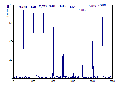
As is typical, the peaks are not centered in the Fourier channels, nor is the displacement of the harmonic from the center of the channel constant. When the displacement is smallest, the amplitudes are highest. Also note that the windowing causes some measure of the spectral information to spread to adjacent channels. That is why the amplitudes in the peak channels are only about 75% of the actual amplitudes of the harmonics.
Click on Cancel and repeat the same steps for the data set Signal B.
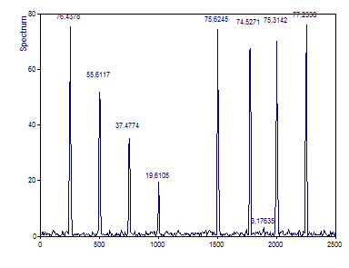
The only apparent difference in the second spectrum is the diminished amplitude of the initial spectral components. Slightly more subtle is the shift in frequency of the sixth and seventh components.
Fourier Cross-Spectra
Click on Cancel to close the Wizard. Select the two data sets Signal A and Signal B by pressing the CTRL key while making the selection.
Click on Insert[Analyses] > Analysis Wizard.
Select the Spectral Analyses category and then Two Signal Spectral Procedures. Next, select Fourier Cross Spectrum. Click on Next.
As with the individual Fourier analyses, for Spectrum Type, select the option Amplitude. For Window Type select the value Cos 3 Minimum Sidelobe -71dB W=3. Make sure that the FFT length is set to the data length or 1024. Select Maximum peak count under Options and enter the value 9. If no labels are visible above the peaks, click on Toggle Labels until the amplitude labels appear.
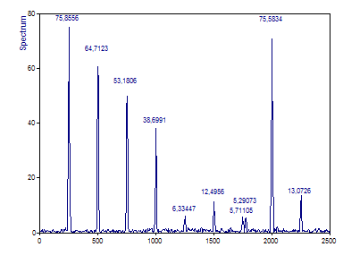
When only the amplitudes vary, as is the case in the second through fourth components, the cross-spectral amplitudes lie between the two spectra.
In the fifth position there is a harmonic in one signal and absolutely nothing in the other. And yet there is still a small peak. This is the cross-spectrum between the high-power signal component in the reference and the noise in the second signal at this particular frequency. Note that the presence of a peak at a given frequency does not allow the inference that there is meaningful harmonic content in both signals. In this case, there is significant harmonic content in only the first of the signals.
In the sixth position we see what happens when two peaks are shifted by only 0.1% of the Nyquist range. There is still a small cross-spectral feature, but it is minor. We are looking at a shift of only 2.5 Hz in a spectrum that covers 2500 Hz.
In the seventh position, the frequency shift is a full 1% of the Nyquist, 25 Hz in this example. There are now two cross-spectral features, one at the central frequency of the component in the first signal, and the other at the central frequency of the component in the second. These are noise peaks in the sense there is no cross-spectral signal content.
If the phase shifts by π , as in the eighth component, it is the same difference as modeling with sines vs. cosines. The full amplitude is recovered. If the phase shift is worst case, however, that of π/2, as in the ninth component, much of the cross-spectral amplitude is lost.
Cross Periodogram
Just as the Periodogram averages individual overlapping segments to produce a reduced variance Fourier estimate at the expense of frequency resolution, so are these same principles applicable to cross-periodograms.
Select the Cross Periodogram algorithm. Make sure that the Amplitude is selected and the Window Type is set to Cos 3 Minimum Sidelobe -71dB W=3. The Segment Length is data length/4 or 256 and the FFT length is set to Segment Length or 256. The Overlap should be 50%. Select Maximum peak count under Options and enter the value 9. If no labels are visible above the peaks, click on Toggle Labels until the amplitude labels appear.
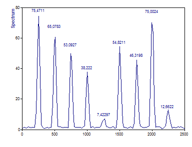
The peaks are much wider because the Fourier resolution is only 1/4 of the single segment cross spectrum. This reduced frequency resolution is a significant factor in this example.
The reduced variance is apparent from the much smoother spectrum. The cross-spectral amplitudes in the initial components are more accurately determined. The cross-spectrum between the harmonic and noise in the fifth frequency position is now a smooth low power peak.
The greatest difference rest with the sixth and seventh components. Due to the reduced frequency resolution, there is now a significant overlap between the components. The 2.5 Hz shift results in a cross-spectral amplitude that is reduced by less than a third. Even the 25 Hz shift results in a reduction of cross-spectral amplitude that is less than half of what would be the case if the frequencies fully matched.
We will now take steps to improve the resolution of the Cross-Periodogram. Since we are not performing high dynamic range cross-Fourier analysis (looking for very low power components that are common), we will use a window that does not cause as much loss in frequency domain resolution. We will also double the resolution by using a segment that is half the data length. To improve the variance, or at least to produce a smoother spectrum, we will average more segments by increasing the overlap.
Set the Window Type to Cos2 Hanning -31dB W=2 , the Segment Length to 512, the FFT length to the Segment Length or 512. Change the Overlap to 90%.
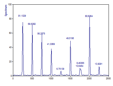
Note that the peaks are much sharper and the cross-spectral peaks are much less in magnitude for the sixth and seventh components that differ in frequency. Some of the smoothness has been lost, but the amplitudes are now somewhat higher due to less spillover into adjacent bins.
Coherence
When multiple segments are used, it is possible to produce a Coherence spectrum. The coherence is 1 when there is similarity in the spectral content at a given frequency and 0 when the signals are dissimilar or fully uncorrelated. This is often a convenient way to look for areas in a spectrum where an output signal is incoherent, that is, having differences in harmonic frequencies.
Select the Coherence procedure and the Coherence spectral type. Leave all of the settings from the Cross-Periodogram intact. Click on Toggle Labels to turn the peak labels off.
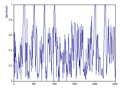
Although the initial components in the two signals differ in amplitude, this does not factor into the MSC, the magnitude-squared coherence. The first four components are shown to have a coherence that reaches 1.
The fifth component, present in one signal and absent in the other, shows nothing above the baseline.
The sixth components, which differ by only 2.5 Hz in frequency across the two signals, have a higher coherence than the seventh components, which differ fully by 25 Hz in frequency. Note also this seventh component produces a consistently low coherence.
The MSC is also phase-independent. The eighth and ninth components produce a coherence of 1, despite the phase shifts.
Signal to Noise Ratio Spectrum
If multiple segments will be used, it is possible to produce a Signal to Noise Ratio spectrum. This uses the coherence values to produce estimates of signal to noise at each frequency in the spectrum.
As the Spectrum Type select Signal to Noise Ratio dB.
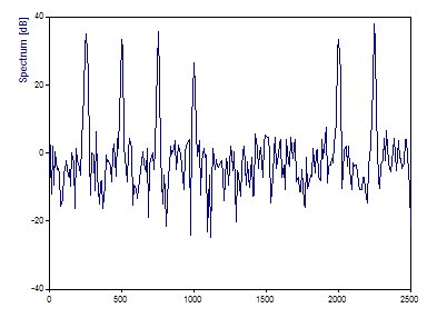
We knew we generated a noise floor at approximately -40 dB on both signals. Here we see peaks that rise about 40 dB above the noise floor. As with the coherence, the components with varying amplitude and phase show full or close to a full S/N. The components shifted 2.5 Hz in frequency show a slight improvement in S/N, but the components shifted by 25 Hz appear indistinguishable from noise. The components shifted by 25 Hz, however, appear indistinguishable from noise.
Transfer Function
The Fourier transfer function is a frequency domain map that represents the transfer properties of a system. In our example, the second signal always contained the same or lesser energy at each of the frequencies except for the two instances where there were frequency shifts.
Unlike the coherence and SNR spectra, a transfer function can be computed with a single segment. As such, we will use the settings we originally applied to the Cross-Spectral procedure.
Select the Transfer Function and the Spectrum Type dB. Select for the Window Type Cos 3 Minimum Sidelobe -71dB W=3. Set the FFT length to data set length or 1024. Click on Toggle Labels to turn the peak labels off. Click on the upper diagram and then on the symbol Activate Cursor (the first one in the toolbox below the diagrams).
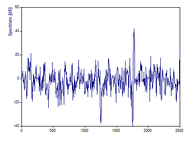
Set the cursor to 250 Hz, which is the position of the first component. The value is approximately 0.17 to 0.18 dB. If you set the cursor to 500, 750, and 1000, you should see -2.5 to -2.6 dB, -6.0 dB, and -11.7 dB.
These correspond with the 1/4, 1/2 and 3/4 reductions in amplitude of these harmonics in the second signal.
Note that there is a deep null in the transfer function at 1250 Hz, where the peak in the second signal is completely absent.
There is also a deep null in the transfer function at 1750 Hz, where again there is no peak in the output signal, and a sharp peak in the transfer function at 1775 Hz, where there is a sharp peak in the output signal, but nothing in the input signal.
Applying a Transfer Function to Input Data
Note for real-world applications it does not make much sense to compute a transfer function from signals of the kind used in the above section. We can easily see that Signal B is not the response of an LTI system because frequencies were shifted, whereas LTI systems change only phases and amplitudes of present spectral components. Further, to get a full picture of an LTI system and thus a well defined transfer function, the input signal needs to stimulate all the modes of the LTI system. Such an input signal would be white noise for example.
To demonstrate this the example project database contains an additional data set called Input Noise and an object called Output Noise, which is a low-pass filtered version of the input noise data. The Transfer Function object has already been set up to compute the transfer function of the signals reflecting this low-pass filter. The diagram with the same name visualizes this. The low-pass filter used is a Butterworth order 4 filter with a cut-off frequency of 100 Hz.
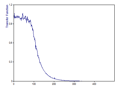
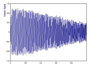
As a final exercise, we will apply the transfer function to an input signal in order to generate an estimate of the output signal. Select the Input Signal object, which is a chirp sine with a frequency ranging from 75 Hz to 125 Hz. Right-click, point to Insert Object and then click on Formula. Enter the following formula: IRFFTn(FFTn('Input Signal') * 'Transfer Function').. Now click on Run to test the formula. You should receive a signal with 1000 points. Click on OK and close the formula window. Highlight the name of the formula again and click on the F2 key). Now enter the new name Output Signal. The formula computes the spectrum of our input signal and multiplies that with the transfer function. This simple computation of the output signal is possible because a convolution in the time domain is equal to a multiplication in the frequency domain. When you multiply the spectra, you need to take care that the frequency count and the frequency spacing is the same for both spectra. To keep this tutorial as simple as possible, we generated our transfer function from a single segment equal to the data length of both the input noise signal and the input chirp signal. If we had averaged overlapping segments, our transfer function would have been both smoother and shorter in length.
We have generated a data set with 1000 real values whose amplitude declines as the frequency goes up. The cut-off frequency of 100 Hz is reached exactly in the middle of our chirp input signal. There, as expected, the amplitude of the output signal is damped about -3 dB.
References
•Oppenheim, A. V. and Schafer, R. W. (1989). Discrete-Time Signal Processing. Prentice Hall, Englewood Cliffs, NJ.
See Also
You might be interested in these articles
You are currently viewing a placeholder content from Facebook. To access the actual content, click the button below. Please note that doing so will share data with third-party providers.
More InformationYou need to load content from reCAPTCHA to submit the form. Please note that doing so will share data with third-party providers.
More InformationYou are currently viewing a placeholder content from Instagram. To access the actual content, click the button below. Please note that doing so will share data with third-party providers.
More InformationYou are currently viewing a placeholder content from X. To access the actual content, click the button below. Please note that doing so will share data with third-party providers.
More Information