Time-Frequency Spectral Analysis Tutorial
This tutorial covers the spectral analysis capabilities of FlexPro for non-stationary data. It covers both the Short-Time Fourier Transform (STFT) and the Continuous Wavelet Transform (CWT). These procedures are useful for studying the changing properties within a data stream as well as identifying stationary regions for conventional Fourier and parametric analysis.
A Test Signal Containing Four Sequential Sinusoids
For this tutorial, we will use a non-stationary data set with four data regions each containing a sinusoid of different frequency.
Select the command File > Open Project Database and open the project database C:\Users\Public\Documents\Weisang\FlexPro\2021\Examples\Tutorials\Spectral Analysis.fpd or C:>Users>Public>Public Documents>Weisang>FlexPro>2021>Examples>Tutorials>Spectral Analysis.fpd. Open the Tutorials folder and its Time-Frequency Analysis subfolder and then double-click to open the 2D diagram called Data.
This is a graph of the signal. There are 1024 floating point values.

The X (time) values vary from 0 to 0.2047 with a 0.0002 sample increment. The Nyquist frequency is thus 2500 (half the 5000 sampling rate). The four sinusoids were generated with the following amplitudes, frequencies, and phases:
100.0*sin(2π*x*1000)+
120.0*sin(2π*x*500+p/2)+
90.0*sin(2π*x*2000+p)+
110.0*sin(2π*x*1500+3p/2)
10% random Gaussian (white) noise was added for a -20 dB noise floor.
The Loss of Time Information in a Fourier Transform
We will begin by exploring a basic Fourier spectrum of this data set.
Close the diagram and highlight the data set Signal.
Click on Insert[Analyses] > Analysis Wizard.
Select the Fourier Analysis category under Spectral Analysis. Next, select Fourier Spectrum. Click on Next.
For the Spectrum Type select Amplitude. For the Window Type select Rectangular -13dB W=1. Make sure that the FFT length is set to FFT length to the data set length or 1024. Select the Maximum peak count option and enter the value 4. Next, set the White Noise Critical Limit % to None. If no labels are visible above the peaks, click on Toggle Labels until the amplitude labels appear.
The Fourier plot in the Analysis Wizard should be as follows:
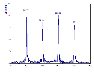
While the Fourier spectrum correctly identifies the frequencies of the four sequential components, there is no indication of where these harmonics begin and end in time. All time-localization information is lost since each component is assumed to be infinite in duration.
Further, since each component is present for only about one-fourth of the overall data length, each amplitude is approximately one-quarter its value in the transient harmonic.
A signal should must be wide sense stationary in order for a Fourier spectrum to be accurate. This means that the spectral content should be constant in both frequencies and powers across the duration of sampling. Both the CWT and the STFT analyses are effective in analyzing non-stationary signals since they furnish a time-frequency spectra of the data.
Short-Time Fourier Transform Spectrum
The Short-Time Fourier Transform (STFT) is similar to the periodogram or segmented-overlapped FFT, except that a central time value is assigned to each segment. Unless there is a need to directly retrieve the amplitude or power from the spectral peaks, a data tapering window is usually used to create the best possible time localization.
Time-frequency spectra are intrinsically fuzzy. The better the resolution in time, the poorer is the frequency resolution. The STFT is the best way to get a good feel for this effect.
Click on Back to go to Step 1 of the Analysis Wizard. Select the Time-Frequency Spectrum and from there STFT. Click on Next to advance to Step 2. The Short-Time Fourier Transform (STFT) procedure is automatically selected.
For the Spectrum Type select dB normalized. Set the Window Type to Cos2 Hanning -31dB W=2. Default values are selected for the starting point. Make sure that the FFT length is set to Segment Length and the Segment Length is at 256, which is equal to 1/4 the data length. Set the Overlap % to 50.
To place time along the X axis, as is typically done with Time-Frequency spectra, check Frequency is Z. Set the Maximum dB range to 20 and keep Maximum STFT frequencies at unlimited.

These settings produce 7 time snapshots, each of length 0.05 seconds. There are 129 frequencies. While there is a sharp definition of the components at the frequencies of 500, 1000, 1500, and 2000, the sequential nature of the four harmonics is obscured by the very poor definition in time. Also, since the time assigned to a snapshot is the mean time in the segment, there is an appreciable zone at the two time bounds where no spectral information is available.
A very simple way to increase the density in time is to increase the Overlap %.
Change the Overlap % to 90.
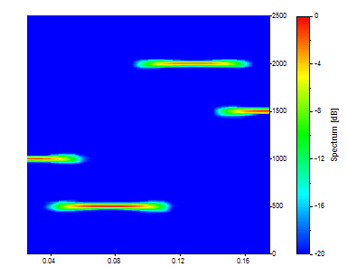
There are now 31 different time snapshots comprising this spectrum. The same 129 frequencies are present. While this produces a modest improvement in time resolution, each snapshot is still an average across one quarter of the data. To improve the time-resolution, it is necessary to decrease the segment length.
To halve the Segment Length, change it to 128. Keep the Overlap % at 90.
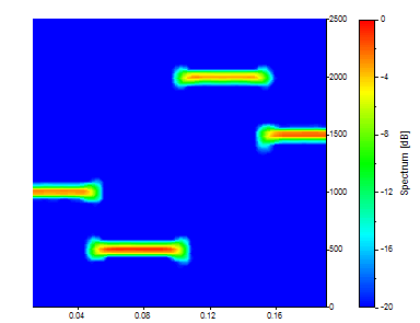
There are now 75 time segments, each an average across one-eighth of the data. There are 65 frequencies. The time-frequency tradeoff should now be apparent. There is now a much stronger definition in time, but the frequency resolution has significantly degraded.
Change the Segment Length to 64. Keep the Overlap % at 90.
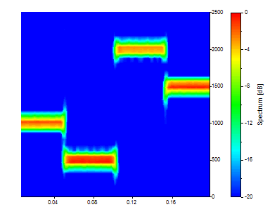
There are now 161 time segments, each an average across 1/16th of the data. There are 33 frequencies. The definition in time is further improved, but the frequency resolution has become significantly fuzzier. Carry this one step further. Change the Segment Length to 32. Keep the Overlap % at 90.
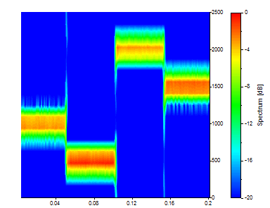
There are now 331 time values but only 17 frequency nodes in the spectral grid. The time snapshots represent averages across 1/32nd of the data and as such the definition in time is quite sharp. On the other hand, the peaks almost meet in the frequency domain.
The visualization is sometimes clearer with a true 3D surface plot.
Click on Standard view. To improve the 3D rendering grid, change the FFT length to 128.
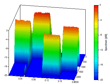
This is a good way to visualize a time-frequency tradeoff that favors resolution in time. We will now return to the initial settings that favored frequency.
Set the Segment Length to 256. Set the FFT length to Segment Length and Overlap % to 90.
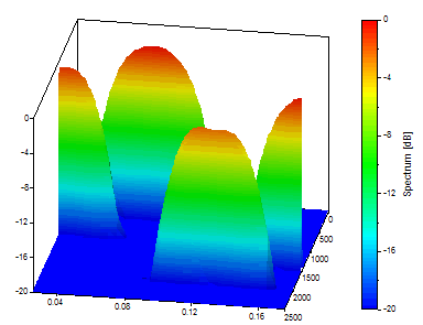
This is a good visualization of a time-frequency tradeoff that favors resolution in frequency at the expense of significant fuzziness in time.
Optimizing the STFT parameters can be challenging. The STFT is a single resolution technique. The same time-frequency tradeoff is present everywhere in the spectrum regardless of frequency. Although the STFT does require careful fine tuning, a spectrum can readily yield spectral amplitudes and powers directly from the height of spectral peaks. Use a tapering window and set Normalization to Amplitude or use a rectangular window combined with high overlap.
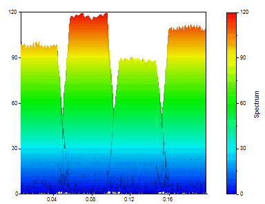
You will get the following graph if you set the Spectrum Type to Amplitude, the window type to Rectangular -13dB W=1 (no windowing), Segment Length to 64, FFT length to 256 and Overlap % to 90.
Continuous Wavelet Transform Spectra
The STFT uses phase-bearing sine basis functions. The infinite duration of sine functions requires the transform of windowed segments of the data stream. If the basis functions were themselves of finite duration, a spectrum could be created from the correlation between shifted and stretched/compressed versions of this limited duration mother "wavelet" and the data stream.
This is the essence of the Continuous Wavelet Transform (CWT).
Despite the awesome array of wavelet shapes, using wavelets for time-frequency spectral analysis is generally easier than optimizing the STFT. And in most instances, the differences between the various mother wavelets and settings do not greatly impact the resulting time-frequency spectrum. The mother wavelet and adjustable parameter selection typically involve selecting a time-frequency tradeoff.
Select Continuous Wavelet Transform (CWT) and dB normalized as the Spectrum Type. Set the Wavelet Type to Morlet and Adjustment (wavenumber) to 8. Set the Zero Pad to 1024 (pad the 1024 data to 2048, the next power of 2), the Number of Frequencies to 40 and keep Start Frequency at 0 and End Frequency at 2500 (the full Nyquist range). Make sure that Frequency is Z is checked, Maximum dB range is set to 20 and Maximum CWT time values is at 1024 (to fully accommodate the 1024 data length).
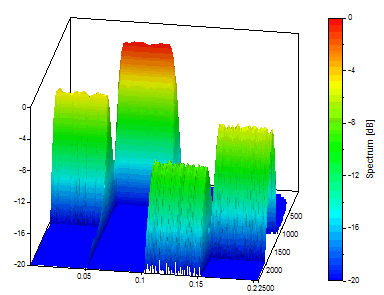
This is a good CWT time-frequency spectrum. In fact, respectable results are attained regardless of the mother wavelet or the value of its adjustable parameter. You could likely use the Morlet wavelet with a wavenumber of 8 for all time-frequency analysis work, and never miss the refinements that would derive from selecting the wavelet whose shape is most compatible with the oscillations in the data and whose oscillation count yields the optimum time-frequency resolution.
To see this fact, we will explore the extremes offered in FlexPro.
For assessing the time-frequency tradeoff in wavelet analysis, we will restore a contour plot. Click on Plan view.
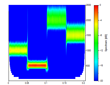
Change the Adjustment to the wavenumber 20.
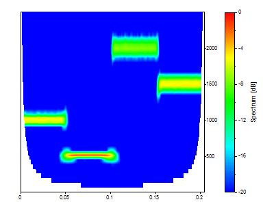
The Morlet with an adjustable parameter (wavenumber) of 20 produces a better frequency localization and a poorer time localization.
Change the Adjustment to 50.
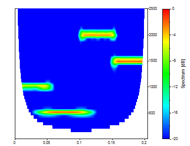
The Morlet with an adjustable parameter (wavenumber) of 50 produces sharp frequency definition but a poor localization in time.
Set the Wavelet Type to Gaussian Derivative and Adjustment to 2.
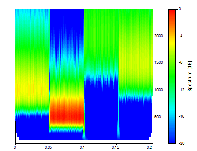
The Gaussian Derivative wavelet with an adjustable parameter of 2 produces the sharpest time localization but as is apparent, very fuzzy frequency localization.
Multiresolution Analysis
The CWT is a multiresolution time-frequency technique. If you inspect the previous plots, you will note that the lowest frequency peak has the highest CWT spectral magnitude and is least smeared in frequency of the four signal components. The highest frequency peak consistently evidences the lowest spectral magnitude and is most smeared in frequency of the four components.
This property is a byproduct of the CWT algorithm rather than a design consideration. Multiresolution analysis has its benefits and drawbacks. If high frequency components are intermittent with a very short time duration, the optimum position would be to tradeoff frequency resolution in order to accurately capture its appearance and disappearance in time. If low frequency components are long-lived, the optimum state would be to tradeoff time resolution for more accurate frequency estimation. When these conditions are true, the multiresolution analysis in the CWT is an asset.
If persistence is independent of frequency, or if the primary aim is to retrieve amplitudes and power directly from the spectral magnitudes, the CWT's multiresolution property is a drawback.
CWT Frequency Redundancy
Unlike the Discrete Wavelet Transform (DWT) traditionally used for wavelet analysis, the CWT can be evaluated at any set of frequencies desired. These frequencies can overlap with an arbitrary measure of redundancy and they can be spaced linearly, logarithmically, or in any sequence. Because a separate FFT must be stored for each frequency evaluated, FlexPro limits the total frequency count to 500. It is this frequency redundancy that allows the CWT to offer a far higher resolution than the DWT.
Again Select the Morlet wavelet. Set a wavenumber of 12. Specify 100 as the Number of Frequencies, 400 as the starting frequency, and 1200 as the end frequency.
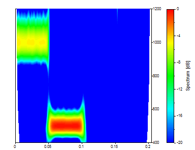
The full analytical power of the CWT spectral analysis is now concentrated in the 400 to 1200 frequency band.
FFT Zero Padding and Edge Effects
Unlike a conventional Fourier analysis where the spectrum is generated by the transform, the FFT is used in the CWT is strictly for performing fast convolution of the scaled and translated wavelet with the data stream. In the CWT the basis functions are scaled and shifted wavelets, not the Fourier sines and cosines. Zero padding has only a single purpose in the CWT, that being to avoid wraparound effects (aliasing) in the fast convolution procedure. Wraparound is fully avoided at all frequencies when the FFT length is twice the length of the data stream. It is often possible to zero pad to the next power of two and avoid any perceptible wraparound and at the same time achieve the fastest possible convolutions.
When an exact N FFT is used for the fast convolution, the wraparound at low frequencies is readily apparent. This wraparound effect diminishes with frequency. This explains the absence of a wraparound effect with the highest frequency component. If there is negligible low frequency content, or if the data are cyclic in the band processed, there is no need to use zero padding.
When zero padding is used to avoid this effect, the power associated with the wraparound is discarded. This results in a diminished power near the edges of the data record. In CWT terminology, this zone where the power may be lessened is known as the cone of influence. The cone of influence is particularly important when the frequency spacing is logarithmic.
Set the Morlet's wavenumber to 100, Zero Pad to 0, Number of Frequencies to 40, Start Frequency to 0 and End Frequency to 2500.
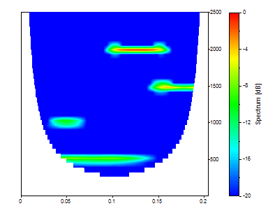
In this case, the very high wavenumber results in a much larger cone of influence. The lowest frequency component actually wraps around to the right of the time scale. This is not shown in FlexPro since information in this cone of influence is not plotted.
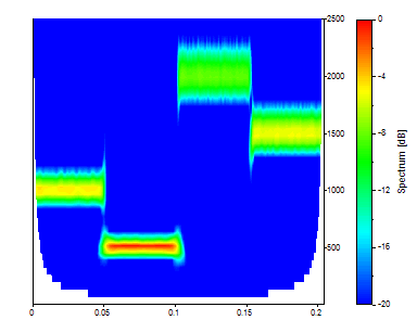
Set the Morlet's wavenumber to 12 and then click on Next. Check both options in Step 3 and click on Finish.
Four total objects are created in the FlexPro project database.
"Spectrum" is the analysis object. This is the object that performs the spectral analysis. The analysis object can be opened by double-clicking on it.
"Spectrum" is the Time-Frequency Spectrum plot generated by the Analysis Wizard. It uses the Spectrum object:
"Data2" is a plot of the original time domain data.
"Time-Frequency" is a document contains the spectral and data plots.
References
A good introduction to digital signal processing is:
•Oppenheim, A. V. and Schafer, R. W. (1989). Discrete-Time Signal Processing. Prentice Hall, Englewood Cliffs, NJ.
•H.D. Lüke (1985). "Signalübertragung (Signal Transmission)". Springer-Verlag Berlin, Heidelberg, New York. ISBN 3-540-15526-0.
The FFT Algorithms used in FlexPro are described in:
•C. Temperton, "Implementation of a Self-Sorting In-Place Prime Factor FFT Algorithm", Journal of Computational Physics, v. 58, p. 283, 1985
•R. C. Singleton, "An Algorithm for Computing the Mixed Radix Fast Fourier Transform", IEEE Trans. Audio Electroacoust., v. AU-17, p. 93, June 1969
•L. R. Rabiner, R. W. Schafer, C. M. Rader, "The Chirp z-Transform Algorithm and Its Application", BSTJ, 48, p.1249, May-June 1969
Information on data tapering windows is given in:
•Albert H. Nuttall, "Some Windows with Very Good Sidelobe Behavior", IEEE Trans. ASSP, v29-1, Feb. 1981.
For those who want to understand the subtleties of applying wavelet analysis to real-world data, there is a well-written paper that covers the CWT in a thorough and accessible manner:
•Christopher Torrence and Gilbert Compo, "A Practical Guide to Wavelet Analysis", Bulletin of the American Meteorological Society, v.79, no.1, p.61-78. January 1998
This reference explains the CWT in the context of analyzing El Nino time series data. The authors have also published a FORTRAN public domain CWT wavelet analysis package WAVEPACK. The document and WAVEPACK code are available at: http://paos.colorado.edu/research/wavelets/.
See Also
You might be interested in these articles
You are currently viewing a placeholder content from Facebook. To access the actual content, click the button below. Please note that doing so will share data with third-party providers.
More InformationYou need to load content from reCAPTCHA to submit the form. Please note that doing so will share data with third-party providers.
More InformationYou are currently viewing a placeholder content from Instagram. To access the actual content, click the button below. Please note that doing so will share data with third-party providers.
More InformationYou are currently viewing a placeholder content from X. To access the actual content, click the button below. Please note that doing so will share data with third-party providers.
More Information