SavitzkyGolayDerivative (FPScript)
Calculates the derivative of a data set with a Savitzky-Golay smoothing filter (least squares derivative). Effective method for determining the smoothed derivative of a noisy data set.
Syntax
SavitzkyGolayDerivative(DataSet, SmoothingWidth, [ PolynomialOrder = 4 ], [ DerivativeOrder = 1 ] [ , Extrapolate = FALSE ])
The syntax of the SavitzkyGolayDerivative function consists of the following parts:
Part |
Description |
|---|---|
DataSet |
The (noisy) data set whose (smoothed) derivative is to be calculated. All data structures are allowed, except scalar value und list. All numeric data types are permitted. If the argument is a list, then the function is executed for each element of the list and the result is also a list. |
SmoothingWidth |
Specifies how many neighboring values, including the respective data point, are to be included in the (smoothed) derivative filter calculation. The smoothing width should be an odd number. Otherwise, the interval is asymmetrical, and one more value is included in the calculation to the right of the center as opposed to the left. Permitted data structures are scalar value. All integral data types are permitted. The value must be greater or equal to 0. If the argument is a list, then the first element in the list is taken. If this is also a list, then the process is repeated. |
PolynomialOrder |
Specifies the order of the polynomial that is fitted locally to the data set and thus used to determine the filter coefficients of the (smoothed) derivative filter.. The polynomial order selected should be less than the smoothing width (so that enough data points are available for local polynomial fitting). Otherwise, the polynomial order is reduced to SmoothingWidth - 1 for the calculation. Permitted data structures are scalar value. All integral data types are permitted. The value must be greater or equal to 1 and less or equal to 15. If the argument is a list, then the first element in the list is taken. If this is also a list, then the process is repeated. If this argument is omitted, it will be set to the default value 4. |
DerivativeOrder |
Specifies the order of the desired derivative. The argument must not be greater than PolynomialOrder. Permitted data structures are scalar value. All integral data types are permitted. The value must be greater or equal to 1 and less or equal to 15. If the argument is a list, then the first element in the list is taken. If this is also a list, then the process is repeated. If this argument is omitted, it will be set to the default value 1. |
Extrapolate |
The value TRUE specifies that the boundary points are to be extended symmetrically for filtering. In this case the filter coefficients only have to be calculated once. Although the extrapolation can lead to an irregular behavior of the (smoothed) derivative at the boundaries, the algorithm remains fast. If FALSE is selected, the same polynomial order is used to determine the (smoothed) derivative at the boundary points. At the boundary points, the smoothing width and the order of the polynomial to be fitted then remain the same, while the filter midpoint is shifted toward the boundaries. The filter coefficients have to be calculated individually for all boundary points in this case. This usually provides higher accuracy for determining the (smoothed) derivative at the boundary points, but the algorithm is considerably slower. Permitted data structures are scalar value. Supported data types are Boolean value. If the argument is a list, then the first element in the list is taken. If this is also a list, then the process is repeated. If this argument is omitted, it will be set to the default value FALSE. |
Remarks
The result has the same structure and unit as the argument DataSet.
To calculate the (smoothed) derivative, each value in DataSet is weighted with (SmoothingWidth-1)/2 left-hand neighboring values and (SmoothingWidth-1)/2 right-hand neighboring values (when SmoothingWidth is uneven). The (smoothed) derivative corresponds to the convolution of the signal with filter coefficients of length SmoothingWidth. For this procedure, the filter coefficients are determined in such a way that the derivative of a local polynomial regression (i.e. local polynomial curve fitting) is returned as the result. The filter coefficients in this case are not dependent on the y values. The algorithm is described in SavitzkyGolay Algorithm.
Filtering is not optimized for the suppression of higher frequencies, but instead is optimized for the suppression of statistic moments of a higher order. The filter is therefore particularly suitable for determining the derivative of signals that, without noise, would have a high frequency range without noise. The Savitzky-Golay smoothing method is also known as "Digital Smoothing Polynomial Filter (DISPO)", "Least-Squares Smoothing" and "Least-Squares Differentiation".
Before filtering, the values are converted into real or complex 64-bit floating point values. The data type of the result is always a real or complex 64-bit floating point value.
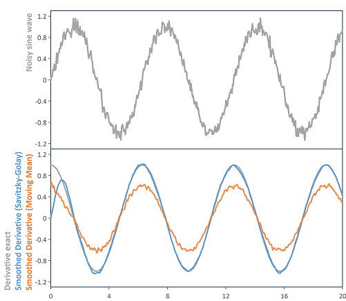
The image highlights the difference of the Derivative function, subsequently smoothed using the Smooth function (moving average), and the SavitzkyGolayDerivative function (with a polynomial order of 7). The same smoothing width is used in each case. The Savitzky-Golay derivative filter can approximate the ideal curve better than the moving average:

Available in
FlexPro Basic, Professional, Developer Suite
Examples
SavitzkyGolayDerivative(Signal, 11, 3)
Calculates the smoothed, first derivative of a noisy signal using the Savitzky-Golay filter. The derivative is calculated by determining the derivative of a third degree polynomial, which is locally fitted to the data set. For local curve fitting a total of 11, i.e. five neighboring values to the left and right of the respective data point, are included in the result.
SavitzkyGolayDerivative(Signal, 25, 6, 2)
Calculates the smoothed, second derivative of a noisy signal using the Savitzky-Golay filter. The second derivative is calculated by determining the derivative of a sixth degree polynomial, which is locally fitted through 25 data points.
SavitzkyGolayDerivative(DataSet, 5, 4)
Calculates the first derivative by determining the derivative of a fourth degree polynomial, which is locally fitted through 5 data points respectively. The fourth degree polynomial, fitted through 5 data points, is uniquely determined and coincides with the Lagrange interpolating polynomial. The calculation result is therefore equal to: Derivative(DataSet, DERIVATIVE_CENTRAL_5_POINTS).
Dim N = 6
Dim polyOrder = 6
Dim width = 2*N + 1
Dim dirac = (0 # width) : 1 : (0 # width)
Dim coeff = SavitzkyGolayDerivative(dirac, width, polyOrder, 1)[N+1, N+ width]
AmplitudeResponse(coeff)
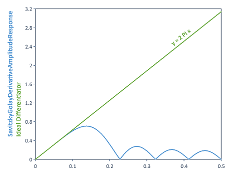
Calculates the amplitude response of the Savitzky-Golay derivative filter (for a polynomial order of 6 and smoothing width of 13). To do this, the SavitzkyGolayDerivative function is applied to a Dirac impulse. This provides the system transfer function in the form of the filter coefficients. With the help of filter coefficients, the AmplitudeResponse function can be used to calculate the filter amplitude response.

See Also
Signal Analysis - Analysis Object
References
[1] Savitzky, A.; Golay, M.J.E.: Smoothing and Differentiation of Data by Simplified Least Squares Procedures. In: Analytical Chemistry, Vol. 36, No. 8, Pages 1627-39. http://pubs.acs.org/doi/abs/10.1021/ac60214a047,1964.
[2] A. Gorry: General least-squares smoothing and differentiation by the convolution (Savitzky–Golay) method. In: Analytical Chemistry, Vol. 62, No. 2, Pages 570-3. http://pubs.acs.org/doi/abs/10.1021/ac00205a007,1990.
You might be interested in these articles
You are currently viewing a placeholder content from Facebook. To access the actual content, click the button below. Please note that doing so will share data with third-party providers.
More InformationYou need to load content from reCAPTCHA to submit the form. Please note that doing so will share data with third-party providers.
More InformationYou are currently viewing a placeholder content from Instagram. To access the actual content, click the button below. Please note that doing so will share data with third-party providers.
More InformationYou are currently viewing a placeholder content from X. To access the actual content, click the button below. Please note that doing so will share data with third-party providers.
More Information