Harmonic Estimation Tutorial
This tutorial covers the spectral analysis capabilities of FlexPro relative to harmonic modeling and harmonic distortion measurements.
Fourier Analysis
If you have not already done so, it is recommended that you go through the Fourier Analysis and Spectral Estimator tutorials before beginning this one. The first step in FlexPro's harmonic estimation is a fully automatic frequency estimation typically accomplished via Fourier analysis, AR spectral analysis, or eigenanalysis.
A Harmonic Test Signal with Distortion and Noise
For this tutorial, we will use one 1024 length signal. There will be one primary harmonic, and a number of secondary harmonics at multiples of the frequency of the primary:
100.0*sin(2π*x*250+p/4)
10.0*sin(2π*x*500+p/2)
1.0*sin(2π*x*750+p)
0.1*sin(2π*x*1000+3p/2)
0.01*sin(2π*x*1250+7p/4)
The sample rate is 5000 Hz, and as such the Nyquist frequency is 2500 KHz, the maximum frequency that can be detected. The time values vary from 0 to 0.2046 at a 0.0002 sample increment. 0.01% random Gaussian noise was added. This produces a noise floor at about -100 dB relative to the largest peak.
Select the command File > Open Project Database and open the project database C:\Users\Public\Documents\Weisang\FlexPro\2021\Examples\Tutorials\Spectral Analysis.fpd or C:>Users>Public>Public Documents>Weisang>FlexPro>2021>Examples>Tutorials>Spectral Analysis.fpd. Open the Tutorials folder and its Harmonic Estimation subfolder and then double-click to open the 2D diagram called Data .
This is a graph of the signal. There are 1024 floating point values.
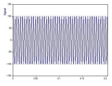
Only the principal harmonic is apparent in time domain. The secondary harmonics represent a very significant harmonic distortion.
Although it is possible to determine the number of harmonic components without doing so, we will first explore the Fourier Spectrum for this signal.
Fourier Spectra
Close the graph window and highlight the Signal data set.
Click on Insert[Analyses] > Analysis Wizard.
Select the Fourier Analysis category under Spectral Analyses. Next, select Fourier Spectrum. Click on Next.
For the Spectrum Type select dB normalized. For the Window Type select Chebyshev and enter 4 for the window's adjustable parameter. Make sure that the FFT length is set to 16384. Select the Maximum peak count option and enter the value 5. Next, set the White Noise Critical Limit % to None. If no labels are visible above the peaks, click on Toggle Labels until the dB labels are displayed.
The Fourier plot in the Analysis Wizard should be as follows:
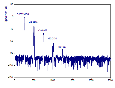
Clearly the secondary harmonics are accurately characterized by the Fourier Spectrum.
Click on Toggle Labels until frequencies are displayed.
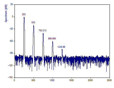
The frequencies of the principal harmonic as well as the secondaries are also accurately estimated from this optimized Fourier spectrum.
Fourier Methods for Frequency Identification
The conditions we have used for the Fourier spectrum represent those that are implemented automatically in the harmonic estimation procedure that uses Fourier analysis for frequency identification. In all cases, the Chebyshev data taper is used and its frequency domain one-sided width is set automatically. For data lengths 256 and less, this width is set to 2. For data lengths above 1024, the window width is set to 4. Between these values, this window adjustment varies logarithmically by -6+1.4427ln(n). This produces a frequency domain width of 3 for a data length of 512. Zero padding is done to create a 16384 length FFT if the data length is less than 16384.
There are two caveats relative to using Fourier analysis for frequency identification. The first is that, even with data tapering, zero padding, and bin-interpolation, the frequency estimation accuracy may be less than the AR or Eigenanalysis procedures. This is particularly true if the data length is in the vicinity of one-thousand points or fewer. Fourier analysis for frequency identification is not recommended if the data length is significantly less, such as a few hundred points.
An equally important issue is that Fourier analysis sometimes produces a sharp spectral feature on the rise and decay of a large spectral peak. The Chebyshev window was selected to minimize this effect, but it may still occur, especially with zero padding implemented to improve the frequency estimates. Since harmonic analysis may include a few harmonics to model trends in the noise, and thus further improve the accuracy of the components modeling signal, it is important that peaks on the shoulders of the principal harmonic not register significantly in the harmonic model.
This is the Fourier Spectrum, exactly as above, except the -92 dB Blackman-Harris window is used and 10 peaks are detected.
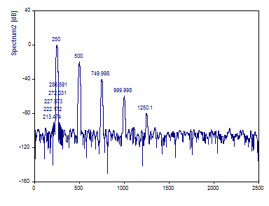
Note that the five additional peaks all occur on the shoulders of the principal harmonic peak. In such an instance, it will not be possible to include additional harmonics to model noise. Instead, it is essential that only five harmonics be included in the model.
Harmonic Estimation
The aim of harmonic estimation is to model a signal with narrowband sinusoids or damped sinusoids. The product of the analysis is a set of harmonics defined by amplitude, frequency, and phase, and also damping factors in the case of damped sinusoids.
Click on Back. Select the Harmonic Analyses category under Spectral Analysis. Next, select Harmonic Estimation. Click on Next. Select for the Algorithm Fourier and for the Model Sinusoid. Set the number of components By maximum count and enter 10. The result type is Harmonic Components. Click on Toggle Labels until the amplitudes are displayed.
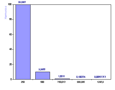
Although it is possible to read the amplitudes from the labels, this is not a good visualization. A logarithmic scale is needed to properly display the wide dynamic range of amplitudes.
Click on Next to advance to Step 3 of the wizard. Check the uppermost check box and then select the 2D Diagram with the name Harmonics. Check the logarithmic Y axis. Click on Back to return to Step 2 of the wizard.
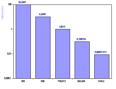
The harmonic modeling algorithm is a two-step procedure. The Fourier step is used only to estimate the frequencies where spectral content is present. The amplitude or power information from the Fourier spectrum is not used in harmonic estimation. In this instance, the Fourier method was used to determine the 10 frequencies with the most significant frequency domain spectral content. The Harmonic Spectrum pictured here is created through a time-domain linear least-squares sinusoidal fit. The first four amplitudes are very accurately determined. The fifth harmonic has an error greater than 10%. The remaining harmonics were intended to model the noise that was present. Since white noise is uniformly distributed across all frequencies, and that is not the case here, the harmonic count should be set to the actual count of signal harmonics.
Although we have good confirmation of the five signal peaks from a visual inspection of the Fourier spectrum, it is not as clear in the harmonic fit based upon the Fourier frequencies. There is no clear demarcation between signal and noise.
Select the AR Data Matrix FB SVD algorithm. Set the model order to 40.
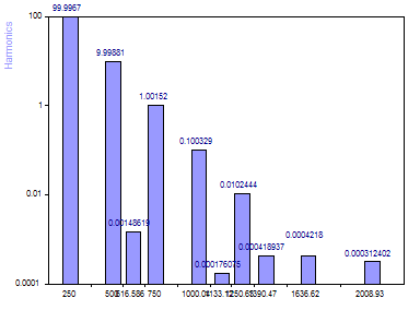
When the AR SVD algorithm is used for frequency identification, there are clearly five components above the noise floor. Further, because the frequencies were more accurately estimated, the amplitudes from the linear sinusoidal fit are also more accurate. Also, the additional harmonics are much more uniformly spread across frequencies, as would be expected in capturing some of the trend in the random noise.
Select the EigenAnalysis Root MUSIC algorithm.
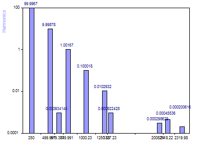
When the Eigenanalysis MUSIC algorithm is used for frequency identification, there are also clearly five components above the noise floor. The accuracy of the amplitudes from the linear sinusoidal fit are very close to that of the AR method.
The AR SVD method strictly uses the signal eigenmodes to estimate frequencies. The Eigenanalysis strictly uses noise eigenmodes to estimate frequencies. Either may be more accurate in any given modeling. It is often a good idea to check both. Note that the five signal frequencies are a near exact match for both procedures. The five harmonics added for modeling the noise have far less overlap.
Parameters of Harmonic Components
White noise should be uncorrelated. This means there should be no trend or persistence. The amplitude of noise at a given discrete frequency should not impact in any way its amplitude at the the next frequency. If noise is perfectly uncorrelated, we will see no benefit from the additional harmonics used for fitting trends in the noise.
To model only the five signal components, set the Maximum count to 5.
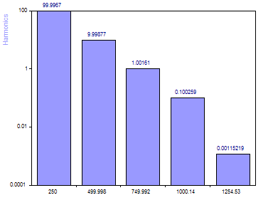
Note that the lowest power secondary harmonic (amplitude 0.01) is no longer estimated accurately. In fact, its estimated amplitude has dropped to nearly one-tenth its true value. Whereas we had five harmonics available to model random oscillations in the noise when we specified 10 harmonics in the fit, we now have only the five actual signal components being fitted. The noise adversely impacts the fit of this least power secondary harmonic.
Set the Maximum count back to 10. Click on Next. In Step 3, select the first two output options and click Finish. Double click on HarmonicAnalysis.
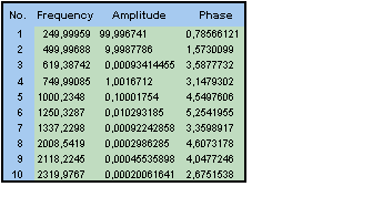
The frequencies, amplitudes, and phases of the five signal components are quite accurately estimated. As is typical in harmonic modeling, the frequencies will have the lowest fractional error, the amplitudes will be next, and the phases will show the highest fractional error. The amplitude errors are in between. The higher the power of any given component, the greater the accuracy will tend to be for the parameters defining that harmonic.
Harmonic Distortion
The THD, or total harmonic distortion, is the ratio of the square root of the sum of the powers or squared amplitudes of all harmonic frequencies above the fundamental frequency to the amplitude of the fundamental frequency.
Traditionally, FFTs were used to measure the THD. Because of spectral content that spills to adjacent bins with windowing, or the spectral leakage that occurs when using an unwindowed Fourier spectrum, it is very difficult to compute an accurate THD using an FFT. This is especially true if noise is to be omitted and only the secondary harmonics are to be included.
FlexPro's harmonic modeling makes it possible to achieve an accurate estimate of the true THD. We know that the correct THD for this test signal is sqrt(10²+1²+0.1²+0.01²) / 100. This is 10.05%.
The settings we used for harmonic modeling are also appropriate for a harmonic distortion spectrum.
Highlight the Signal data set.
Click on Insert[Analyses] > Analysis Wizard.
Select the Harmonic Analyses category under Spectral Analysis. Next, select Harmonic Estimation. Click on Next.
Select the Algorithm EigenAnalysis Root MUSIC and Model Sinusoid. Set the number of components By maximum count to 5. For the Spectrum Type select Harmonic distortion spectrum %. Click on Toggle Labels until the % of distortions are displayed.
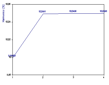
The number of components are shown on the x-axis. At component 2, the harmonic distortion between the first secondary harmonic and the principal component is plotted. At component 3, the harmonic distortion associated with the first and second secondary harmonics is plotted. Thus the THD (absent noise) is the value at component four. The value of 10.0497 is very close to the 10.0504 value we know to be correct. If you set the number of components to 10 again, you will see that additional noise components do not contribute substantially to the THD.
Click on Finish to close the Analysis Wizard.
See Also
You might be interested in these articles
You are currently viewing a placeholder content from Facebook. To access the actual content, click the button below. Please note that doing so will share data with third-party providers.
More InformationYou need to load content from reCAPTCHA to submit the form. Please note that doing so will share data with third-party providers.
More InformationYou are currently viewing a placeholder content from Instagram. To access the actual content, click the button below. Please note that doing so will share data with third-party providers.
More InformationYou are currently viewing a placeholder content from X. To access the actual content, click the button below. Please note that doing so will share data with third-party providers.
More Information