MeshGrid (FPScript)
Produces a two-dimensional grid. Helpful for three-dimensional visualization of functions with two variables or functions with complex-valued arguments.
Syntax
MeshGrid(X, Z)
The syntax of the MeshGrid function consists of the following parts:
Part |
Description |
|---|---|
X |
Defines the horizontal dimension (X direction) of the two-dimensional grid. Permitted data structures are data series. All numeric data types are permitted. |
Z |
Defines the vertical dimension (Z direction) of the two-dimensional grid. Permitted data structures are data series. All numeric data types are permitted. |
Remarks
The result always has the data structure list.
From two data series, X with length N and Z with length M, the function produces a list with two entries bearing the same names: X and Z. However, the resulting entries in the list are now matrices consisting of N rows and M columns, which are formed by replicating the function arguments X or Z. The units of the result matrices match the units of the individual arguments.
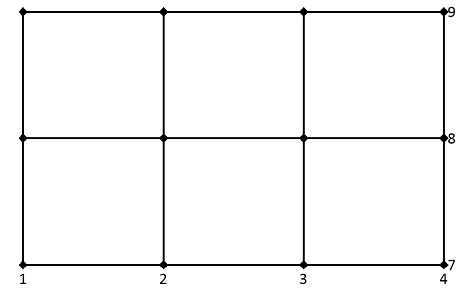
The result can be interpreted as a two-dimensional rectangular grid with N x M grid points as follows: For example, specified are the data series X as {1, 2, 3, 4} in the horizontal direction and the data series Z as {7, 8, 9} in the vertical direction. The grid spanning from X and Znow comprises the coordinates (1, 7), (2, 7), (3, 7), (4, 7), ..., (1, 9), (2, 9), (3, 9), (4, 9):

The coordinates of the individual grid points are obtained on a per-element basis from the two matrices bearing the same names:
The function MeshGrid applied to the two data series, now results in the list consisting of the matrices bearing the same name X (first list element) and Z (second list element).
The function is usually used for the three-dimensional display of the functions y = f(x, z) of two variables over a two-dimensional rectangular grid. In particular, functions y = f(z) = f(z1, z2) with complex-valued arguments z = z1 + i * z2 can be calculated and displayed over the complex plane.
Available in
FlexPro Basic, Professional, Developer Suite
Examples
Dim x = {1, 2, 3, 4}
Dim z = {7, 8, 9}
Dim grid = MeshGrid(x, z)
Dim y = grid.["X"]^2 - grid.["Z"] // = grid.[0]^2 - grid.[1]
Signal(y, x, z)
Example 1: Procedure for calculating functions with two variables
Calculates the function y = x^2 - z spanning the grid using the data series {1, 2, 3, 4} (in the X direction) and {7, 8, 9} (in the Z direction):

Dim x = Series(-4, 4, 0.01)
Dim z = x
Dim grid = MeshGrid(x, z)
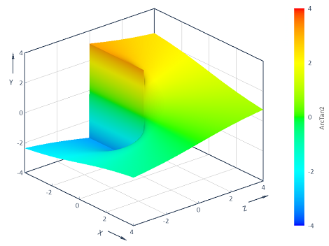
Dim y = ArcTan2(grid.["Z"], grid.["X"])
Signal(y, x, z)
Example 2: Visualization of the ArcTan2 function with 2 variables
Calculates the ArcTan2 function y = f(x, z) = ArcTan2(z, x) across the two-dimensional (x, z) range [-4, 4] x [-4, 4]. The visualization in a 3D contour diagram results in the following:

Dim x = Series(-16, 16, 0.04)
Dim z = x
Dim grid = MeshGrid(x, z)
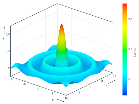
Dim y = Sinc(Sqrt(grid.["X"]^2 + grid.["Z"]^2))
Signal(y, x, z)
Example 3: Visualization of the Sinc function in 2D
Calculates the two-dimensional Sinc function y = f(x, z) = Sinc(Sqrt(x^2 + z^2)) across the two-dimensional (x, z) range [-16, 16] x [-16, 16]. The visualization in a 3D contour diagram results in the following:

Dim z1 = Series(-6, 6, 0.02)
Dim z2 = z1
Dim grid = MeshGrid(z1, z2)
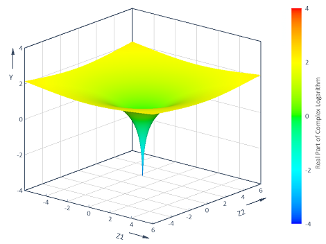
Dim y = Real(Log(grid.[0] + 1i * grid.[1]))
Signal(y, z1, z2)
Example 4: Visualization of functions with complex arguments
Calculates the real part of the complex logarithm y = f(z1, z2) = Real(Log(z1 + i* z2)) across the complex (z1, z2) plane [-6, 6] x [-6, 6]. The visualization in a 3D contour diagram results in the following:

Arguments x, z
Dim xMatrix = x # NumberOfRows(z)
Dim zMatrix = TransposeMatrix(z # NumberOfRows(x))
List("X", xMatrix, "Z", zMatrix)
Example 5: Equivalent FPScript code
The following FPScript code produces the same result as the MeshGrid function.
