This tutorial covers non-linear curve fitting in FlexPro for particular cases in which the input signal has multiple peaks. If you have not already done so, it is recommended that you go through the Non-Linear Curve Fitting Tutorial first before beginning this one. Most of the principles of non-linear curve fitting are covered in that tutorial.

Example 1

Select the command File > Open Project Database and open the project database C:\Users\Public\Documents\Weisang\FlexPro\2021\Examples\Tutorials\Curve Fitting.fpd or C:>Users>Public>Public Documents>Weisang>FlexPro>2021´>Examples>Tutorials>Curve Fitting.fpd. Open the Peak Fitting folder and select the Gauss1 data set.

Click on Insert[Analyses] > Analysis Wizard.

Select the Curve Fitting category and then Peak Fitting. Click on Next.

You can set the baseline function on the first page of the Analysis Wizard. There are several baseline models available. Select Square function as the Baseline. To determine the baseline, several points must be selected on the input signal. Next, the selected linear model will be approximated on the defined points according to the method of least mean square error.

The points can be determined automatically or can be entered manually.

Determining the Baseline Automatically

Select Automatically and enter 30 as the Number of points.

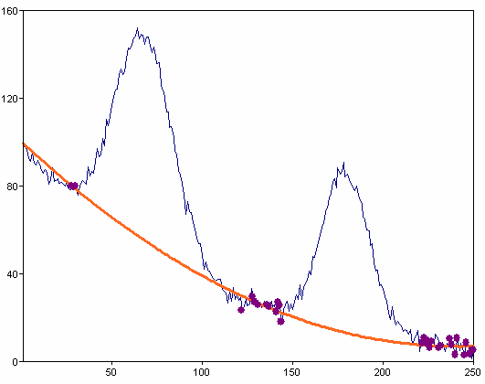
In this case, the points will be determined using a special algorithm. The algorithm selects the points whose first and second derivative oscillate in a particular range round the value 0.

Determining the Baseline Manually

In this method, you can select the precise points to be used for determining the baseline. To do this, select Manually. Now the cursor will be activated in the diagram view. Use the cursor to move to the first point of the baseline to be calculated. Set a marker (Enter key). Repeat this process until you have marked a sufficient number of points. The points must not be on the curve. If you disable the option Bind Cursor To Curve you can also select points next to the curve.

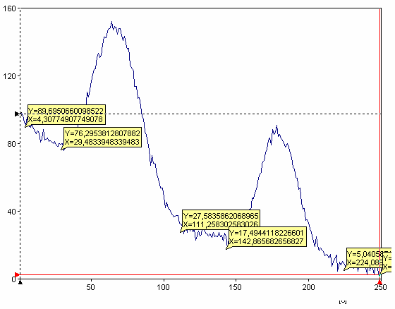
Now press the Calculate Baseline button.

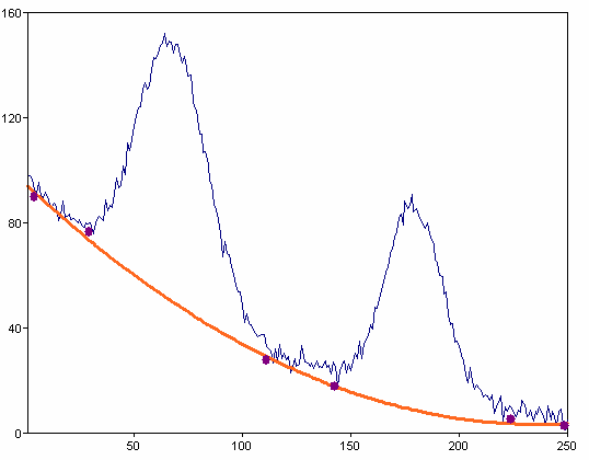
You can also delete the points and baseline by pressing Delete Baseline.

You can now include the calculated baseline in the model as a variable or static component. In the first case, the baseline model parameter values calculated here are adopted as initial values and in the second case, they are adopted as fixed values. Alternatively, you can subtract the baseline from the input signal and apply the non-linear curve fitting to the result. The baseline model is not added to the peak model in this case.

Select Include baseline as variable component into the model for the result and press Next.

Curve Fitting

Non-linear curve fitting is carried out on this page. Select the Model Gauss model (variant 2), 100 as the Maximum number of function calls and choose Manually for the calculation method. In this case, you need to specify the peaks by setting markers as you do when determining the baseline. Define two peaks in this case.

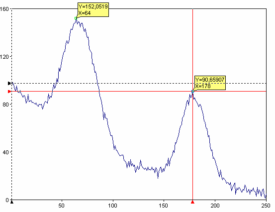
Now press Calculate.

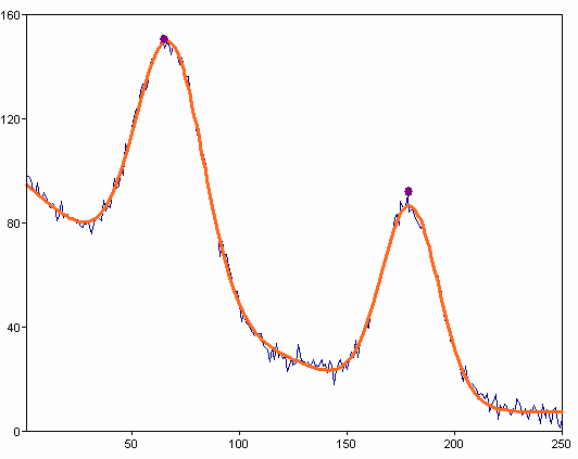
Press Delete Peaks.

Setting Peaks Automatically

Select Automatically and enter 2 as the Number of peaks, 20 as the Hysteresis and Maxima as the Type. During automatic peak search, the program searches for N (number of peaks) local maxima and/or local minima. The hysteresis specifies the minimum amount by which the signal amplitude must rise or fall once a local maximum or minimum has been recognized in order for it to be accepted as a local extreme.

You can also display additional information by enabling the particular option. For instance, you can display the determined peak curves by enabling the Peak curves option.

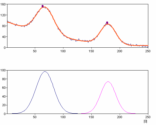
Press Finish to create the analysis object.

Example 2

Select the data set Gauss2.

Select the command Insert[Analyses] > Analysis Wizard.

Select the Curve Fitting category and then Peak Fitting. Click on Next.

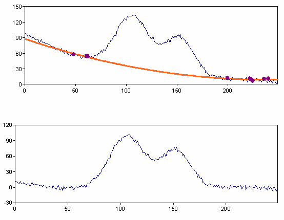
Select Quadratic function, automatic calculation using 10 points and as the Result select Subtract baseline from source data.

On page 2 of the Wizard, select Gauss Model (Variant 2) as the Model, 1000 as the Maximum number of function calls, automatic calculation, 2 for the Number of peaks, 10 for the Hysteresis, Maxima for the Type and then select the Peak curves option.

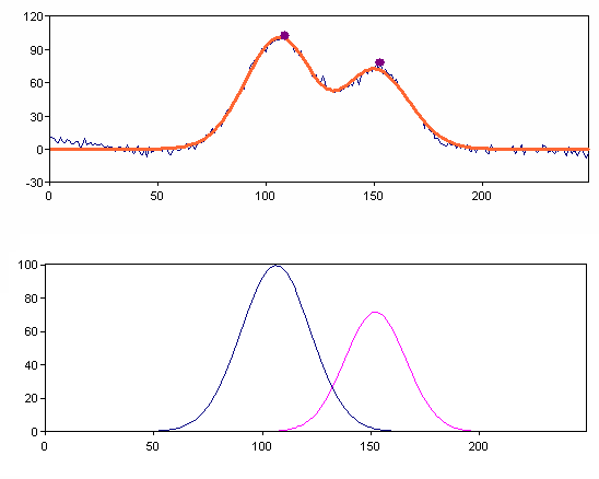
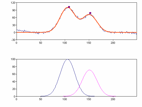
The objective now is to find the best model where both peak curves have the same width. To do this, go to the next page of the Analysis Wizard. In the list of parameters, for the Width parameter, set the option Shared to Yes.

The diagram below shows the determined peaks: