Revolution Synchronous Sampling Analysis Object (Order Tracking Option)
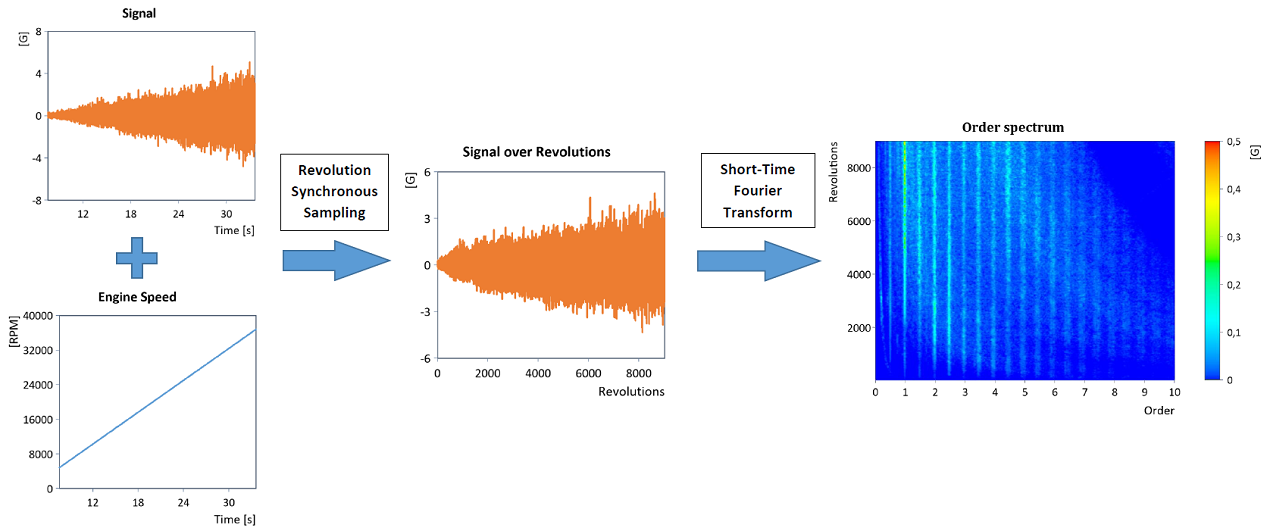
The Revolution Synchronous Sampling analysis object transforms a signal sampled over time into the revolution domain. The signal is then no longer available in temporally equidistant steps, but in equidistant rotation angle steps (i.e. equidistant rotation intervals). In the referenced literature this is referred to as a Synchronous Angular Sampling, Computed Order Tracking, Synchronous Sampling or even Adaptive Resampling.
This provides an effective method for performing order tracking, since the frequency spectrum (i.e. the Fourier Transform) of the signal converted to the revolution domain provides the order spectrum directly:
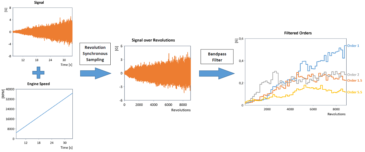
In the same way, ordinary band pass filtering (e.g. using a suitable IIR bandpass filter) can be used to determine the curve of individual orders in the revolution domain (shown here is the blockwise RMS curve of the filtered orders):
Note: the Fourier analysis in the revolution domain (e.g. calculation of an order spectrum) as well as bandpass filtering in the revolution domain can be performed directly in a single step with the Revolution Synchronous Order Tracking and Order Filter analysis objects.
Data tab
This tab specifies the input data in the time domain (for more information, also see RevolutionSyncSampling):
Signals in the time domain
The time signal to be analyzed for the analysis object must be in the data structure Signal. The Speed can either be stored in the Signal data structure (corresponds to run-up or variable speed) or as a scalar value (corresponds to constant speed or fundamental frequency).
If there are no units or unit management is switched off, the speed is always interpreted in the unit [1/min] and the X component of the time signal is interpreted in the unit .
The instantaneous speed is often measured with a pulse encoder, which records a certain number of pulses per revolution. You can convert the resulting pulse signal directly into a speed signal. To do this, select the option Speed is an impulse signal and specify the Number of impulses per revolution. The conversion of the pulse signal into a speed signal is done with the ImpulseToFrequency function.
Options tab
This is the tab where the parameters for transformation from the time to revolution domain are specified. Schematically, the algorithm of the transformation process can be described as follows (for more information, also see RevolutionSyncSampling):
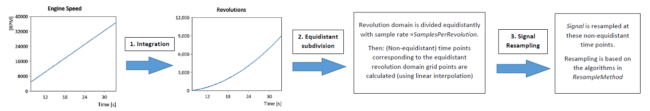
Resampling into the revolution domain
Three different modes are available for resampling from the time to the revolution domain. In most practical applications, the linear resampling is sufficient:
Resampling method |
Description |
|---|---|
Linear interpolation |
The time signal is evaluated at the (non-equidistant) time points of the equidistant revolution sampling points by means of linear interpolation before being transformed into the revolution domain. This makes the transformation fast, but can cause aliasing in the subsequent FFT analysis of the revolution-based synchronous sampled signal. |
Spline interpolation |
The time signal is evaluated at the (non-equidistant) time points of the equidistant revolution sampling points by means of spline interpolation before being transformed into the revolution domain. Compared to linear resampling, spline interpolation is slightly slower, but aliasing is reduced. |
FFT resampling |
The time signal is evaluated by FFT resampling at the (non-equidistant) time points of the equidistant revolution sampling points before being transformed into the revolution domain. Here, the time signal is first transformed into the frequency domain, where zeros are appended and then transformed back into the time domain. Resampling by means of Fourier transform leads to an almost ideal result, since this does not add any high-frequency signal components. Alias effects in the calculation of the order spectrum are almost absent, but the calculation time increases significantly. |
If the splines or the FFT resampling method is selected, a resample factor must be specified by which the sampling rate of the signal is increased during the transformation algorithm.
Regardless of the resampling method selected, the Number of data points per revolution for the signal transformed into the revolution domain must be specified. This determines the sampling of the transformed signal in the revolution domain. According to the Nyquist sampling theorem half of the value determines the maximum order that can even be calculated using Fourier analysis.
To determine the Number of data points per revolution two modes are available:
Data points per revolution |
Description |
|---|---|
Automatic (adaptation to max. order) |
Calculates an automatic value for the number of data points per revolution so that the theoretically largest order occurring in the signal can still be calculated using Fourier analysis. The automatically calculated value can be limited by a freely adjustable limit value. |
Fixed value |
For the number of data points per revolution, any fixed value can be specified. |
Detrending in the revolution domain
In many application examples, an existing, exceedingly large DC offset leads to a visually unsuitable representation in the contour plot of the order spectrum, in which the DC component dominates. It is therefore advantageous to filter out the DC component. For this purpose, for the signal transformed into the revolution domain, a corresponding DC offset high pass filter with adjustable cut-off frequency (cut-off order) and filter order (filter steepness) is set (for details about the DC offset high pass filter, see the DCRemovalFilter function).
Output in the revolution domain
The signal transformed into the revolution domain, the speed data set transformed into the revolution domain or the time component transformed into the revolution domain can be returned. Any combination of these output options are also permitted, which are then combined in the data structure list.
Examples
In the project database C:\Users\Public\Documents\Weisang\FlexPro\2021\Examples\OrderT racking Analysis.fpd or C:>Users>Public>Public Documents>Weisang>FlexPro>2021\Examples\Order Tracking Analysis.fpd you will find examples of the different use cases and modes for which an order analysis can be performed. In particular, the diagrams above are included there.
FPScript Functions Used
See Also
Revolution Synchronous Order Tracking Analysis Object
You might be interested in these articles
You are currently viewing a placeholder content from Facebook. To access the actual content, click the button below. Please note that doing so will share data with third-party providers.
More InformationYou need to load content from reCAPTCHA to submit the form. Please note that doing so will share data with third-party providers.
More InformationYou are currently viewing a placeholder content from Instagram. To access the actual content, click the button below. Please note that doing so will share data with third-party providers.
More InformationYou are currently viewing a placeholder content from X. To access the actual content, click the button below. Please note that doing so will share data with third-party providers.
More Information