Non-linear curve fitting makes it possible to converge a model function dependent on an independent variable and several parameters toward a given data set. This analysis object is primarily used for determining model parameters so that the selected model is adapted to the data in the best way possible. Here, it is essential to have precise knowledge about the selected model and its parameters. The non-linear curve fitting, however, can be used to interpolate or smooth a given data set. In this case, it is not critical as to which model is to be used for the analysis. Likewise, testing the calculated model parameter occurs. For this area of application, a tool that compares the available models to one another (model ranking) is useful.

Example:

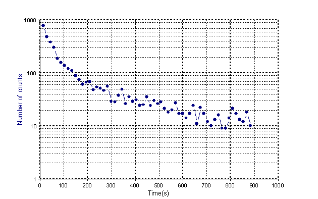
A piece of silver is irradiated to generate two short-lived silver isotopes 47Ag108 and 47Ag110, which then undergo beta radiation once more. For the experiment, the radiated beta particles are counted in 15s intervals for a period of 4 minutes. The result is a decreasing exponential curve that is described by the Exponential decay function (variant 2) model function. The parameter p0 corresponds to the background radiation and p1 and p3 correspond to the amplitudes of both excited states with the mean lives p2 and p4 respectively. Since the model is non-linear in parameters p2 and p4, a method for non-linear curve fitting is required.

Select the command File > Open Project Database and open the project database C:\Users\Public\Documents\Weisang\FlexPro\2021\Examples\Tutorials\Curve Fitting.fpd or C:>Users>Public>Public Documents>Weisang>FlexPro>2021>Examples>Tutorials>Curve Fitting.fpd. Open the folder called Silver Example and then double-click to open the 2D diagram called Ag-Diagram.

This is a diagram for the Ag signal with 59 floating point values. (Source: Bevington, p. 142 ff)

Model Ranking

Close the diagram and highlight the Ag data set, the signal to be analyzed for the experiment described above.

Click on Insert[Analyses] > Analysis Wizard.

Select the Curve Fitting category and then Non-Linear Curve Fitting. Click on Next. Click on Model Ranking to determine which model best applies to the selected data set.

A dialog box opens where you can choose the algorithm, maximum number of function calls and model categories. You can find assignment of individual model functions under Models. For the algorithm select Full Newton. Set the Maximum function calls to 300 and highlight all categories. The higher the value you select for the Maximum function calls, the more models will be returned a result. The time required for calculating the algorithm will, however, increase accordingly. Click on Next.

Now a non-linear curve fitting will be carried out for all selected models and the models based on the absolute residual sum of squares SSE will be sorted and listed. You can choose the model from the list that you want to continue to use. The coefficient of multiple determination R2 will also be listed. R2 = 1.0 means that the curve goes through each data point. With a known X value, the associated Y value is determined precisely. R2 = 0.0 means that the regression model does not describe the data any better than as a horizontal line through the mean value of the data. Known X values are no help when calculating the associated Y value.

Select the model with the smallest absolute square sum of residuals, the NIST model Hahn1 model, to obtain the closest possible convergence. Now close the Model Ranking dialog box by clicking on Finish. Click Nexttwice. Enable the option Diagrams and tables presenting the results. Next, click on Finish.

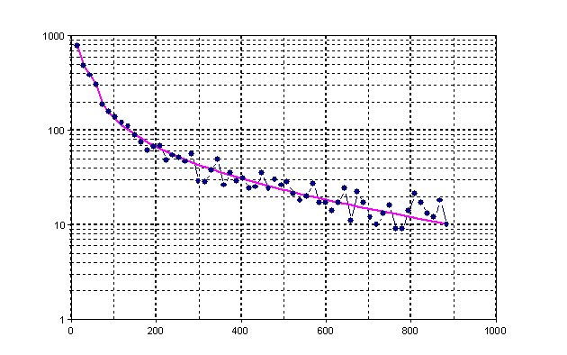
Open the newly created diagram Signal to view the result of the signal smoothing. The following diagram shows the result in logarithmic scaling.

Linear Approximation

Before the model parameters are determined using the non-linear curve fitting, the signal to be analyzed is reduced and transformed in such a way that a linear approximation to determine the model parameters can be used. This method can be used to calculate the initial parameters. In many cases, the selection of initial parameters is a decisive criterion for successful calculation of the model parameters using non-linear curve fitting. The result of linearization in this case serves as a validation check of the non-linear curve fitting result.

The model function to be examined, Exponential decay function (variant 2), has the following format:

First, the background radiation (parameter p0) is determined. One look at the signal curve suffices for a rough estimate. The exponential curve approximates the offset to be determined. To obtain a rough estimate of the background radiation, the last three signal values are averaged. This results in the value 13.3. To determine additional parameters, the offset is subtracted from each point of the signal. The calculated signal is reduced to two partial segments A (x < 120) and B (x > 200). The parameters p3 and p4 are now approximated via a logarithmic transformation and a linear approximation.

Based on this result, the long-lived component can be determined. Now this part is subtracted from Segment A to determine the short-lived component. Here, a logarithmic transformation and a linear approximation also occur.

The parameters determined are as follows:

Open the Linearization formula from the Example Silver folder to view the FPScript function for this calculation.

Estimating Parameters

After this rough estimate of the parameters, you can start determining the precise model parameters.

To do this, select the signal Ag.

Click on Insert[Analyses] > Analysis Wizard.

Select the Curve Fitting category and then Non-Linear Curve Fitting. Click on Next. Select the model Exponential decay function (variant 2). In addition, you can display a prediction band (95%, 99% or 99.9%) and a confidence band (95%, 99% or 99.9%). The confidence band is useful for repetitive data, i.e. for each X value there are several Y values or there is a Y value that represents the mean of several measured points. A 95% confidence interval is the Y range for a given X value that contains the true Y value with 95% probability. The prediction band makes a statement about the scattering of the data to be analyzed. If you were to collect more data points, 95% of the points would fall within the range of the prediction band.

After you have selected the model, you can look directly at the result of the non-linear curve fitting in the Preview pane of the Wizard. In the first diagram, the input signal and the estimated signal are displayed. In another diagram, the residuals are displayed. In both tables you will find the estimated parameters and a number of statistical values for the analysis result. The model parameters calculated have the values:

In this case, p1 and p2 are the parameters for the long-lived components, and p3 and p4 are the parameters for the short-lived components.

Click Next. On this page of the Wizard, various settings are available that can affect the calculation. Select an algorithm. In addition, diverse weighting and scaling modes can be used.

The most important setting option on this page is the Initial Values list. Here, you can determine the initial values of the model parameters. In addition, you can determine whether a parameter has a fixed value or not. For the Full Newton algorithm, an upper and lower bound can be specified as well.

Selecting the initial parameter is decisive in calculating the result. If the selected starting point is far away from the global minimum, the algorithm may not return a result or may return a different local minimum. To increase the probability that a global minimum is in the result displayed, the calculation should be carried out with different initial values. For models with four or fewer parameters, the Estimate Initial Parameters option is available. For each parameter, 10 randomly distributed values are calculated that are found in the range determined by the upper and lower bounds. For each combination, the absolute residual sum of squares is now calculated. The combination with the least square mean sum provides the initial values. The initial parameter values can also be calculated using an FPScript formula. The termination criteria for the algorithm can be affected by the settings options Maximum function calls, X Tolerance, Y Tolerance, F Tolerance and G Tolerance. The calculation of the first iteration depends on the step bound settings.

On the last page of the Wizard, you determine which diagrams, tables and documents are to be set up in addition to the analysis object for the evaluation. Select the option Diagrams and tables presenting the results to generate the diagrams and tables displayed in the Preview pane. If you want to display the Covariance Matrix, Correlation Matrix, Standard Error of the Parameters and the Confidence Intervals of Parameters in table format, select the extra option Optional numeric results. Click on the Finish button to close the Wizard.

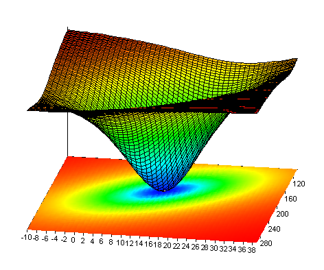
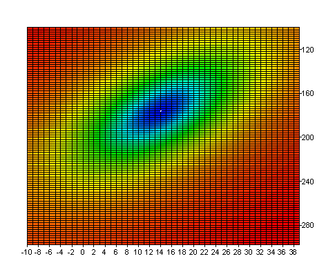
Now, to illustrate that a local minimum is present in the result, in the Surface formula, the Absolute Residual Sum of Squares is calculated for the model. The parameters p0 and p1 are variable; the parameters p2, p3 and p4 are fixed. The result is displayed in the Surface surface diagram. It is important to note that the minimum is at p0 = 14 and p1 = 176.

Using Start Script

This example illustrates how you can use Start Script to calculate the initial values of the model parameters.

Open the Linearization formula described above, select the content of the formula (CTRL+A) and copy the content to the system's clipboard (CTRL+C). Select the signal Ag.

Open the Wizard for the non-linear curve fitting and go to the third page of the Wizard. Click on the button. Paste the script code from the clipboard to the input field (CTRL+V). Click on Calculate to test the script. The result is a data series with five 64-bit floating point values. Click on Apply to accept the calculated values as the initial values. If the number of calculated values does not equal the number of model parameters, the calculated values will not be applied. Instead of directly pasting the script code into the input field, you can refer to a formula that has already been created by entering the name of the formula in the input field. However, the code is then only valid as long as the formula object exists.

Custom Model

In addition to the pre-defined models, it is possible to define your own model functions and determine how to save them. The following example illustrates how to set up a custom model. Select the command File > Open Project Database and open the project database C:\Users\Public\Documents\Weisang\FlexPro\2021\Examples\Tutorials\Curve Fitting.fpd or C:>Users>Public>Public Documents>Weisang>FlexPro>2021 >Examples>Tutorials>Curve Fitting.fpd. Open the folder called Custom Model and double-click to open the Data formula. The formula calculates a signal using the polynomial function y = p0 + p1x + p2x² + p3x³. This is a signal with 1000 64-bit floating point values.

Since this model function is linear, the parameters can be calculated using the Approximation FPScript function (Linear Approximationformula).

To determine the parameters using non-linear curve fitting, select the Data formula and click on Insert[Analyses] > Analysis Wizard. Select the Curve Fitting category and then Non-Linear Curve Fitting. Click on Next. In the Model field, type the name Poly3 for a custom model. Two input fields will appear where you enter the formulas for the model function or the formula for the partial derivatives of the model function. Type p[0] + p[1] * x + p[2] * x^2 + p[3] * x^3 into the function text box. p[0] to p[3] describe the particular model parameters. In the number of parameters list box, select the value 4. Click on Save Model to save the model under the specified name. If an error message appears in the Preview pane instead of the desired results, you will have to increase the Maximum function calls on the next page of the Wizard. Click on Next. Select 300 function calls.

Click on the Back button. To ensure that the partial derivatives are not numerically calculated, but are analytically calculated instead, you have to enter the formulas of the partial derivatives into the Derivatives text box: [ 1, x, x^2, x^3 ]. The partial derivatives must be provided as a list. The result of the estimated model parameters is now more precise. In addition, the required number of iterations is reduced considerably using the Full Newton algorithm through the analytical calculation of partial derivatives. Click on Save Model to resave the model.

You can also assign the parameters names. These names will then appear in the Initial Values list on the next page of the Wizard. To do this, you need to change the formula, which describes the custom model function, in the following way:

Dim p0 = p[0]
Dim p1 = p[1]
Dim p2 = p[2]
Dim p3 = p[3]
p0 + p1 * x + p2 * x^2 + p3 * x^3

The variable p0 is assigned to the variable p[0], and variable p1 is assigned to p[1], etc. Make sure that the assignments are made one below another. Click Next to view the Initial Values list with the renamed parameters.

Click on Finish to close the Wizard.

References

•P.R. Bevington, D.K. Robinson. Data Reduction and Error Analysis for the Physical Sciences, 3rd Ed., McGraw-Hill, New York, 2003.

•G. A. F. Seber, C. J. Wild. Nonlinear Regression. Wiley, New York, 2003.

•Harvey Motulsky, Arthur Christopoulos. Fitting Models to Biological Data Using Linear and Nonlinear Regression: A Practical Guide to Curve Fitting. Oxford University Press, 2004.

See Also

Analysis Wizard

Non-Linear Curve Fitting Analysis Object

Statistical Output Options for Non-Linear Curve Fitting

Non-Linear Models