Statistical Output Options for Non-Linear Curve Fitting
The convergence criteria alone, however, are not sufficient to determine the result of the non-linear curve fitting. A number of statistical quantities are available to help you determine the goodness-of-fit.
Quantity |
Calculated Using |
Note |
|---|---|---|
Estimated Values / The data modeled |
|
You can obtain the estimated values by calculating the selected regression model with the estimated p parameters. |
Residuals |
|
The residuals are the vertical difference between the actual data values and the particular estimated values. If the value is positive, then the corresponding point lies above the estimated curve. If the value is 0, then the point lies on the curve. |
Average Residual |
|
This is the mean value of the residuals. |
Sum of Residuals |
|
The sum can be 0 despite many positive and negative residuals. |
Absolute Residual Sum of Squares |
|
|
Relative Residual Sum of Squares |
with |
This function is often also described as the χ2 function and is a measurement for the goodness-of-fit. |
Regression Square Sum |
|
|
Total Sum of Squares |
|
SST = SSE + SSR |
Error Variance |
|
|
Coefficient of Multiple Determination R2 |
|
R2 = 1.0 means that the curve goes through each data point. With a known x-value, the associated y-value is determined precisely. R2 = 0.0 means that the regression model does not describe the data any better than as a horizontal line through the mean value of the data. Known x-values are no help when calculating the associated y-value.
Only evaluating the R2 value is not enough to interpret a model. The best curve fitting is useless if the parameters determined do not make sense physically and/or the confidence interval is too wide.
|
Adjusted Coefficient of Multiple Determination Ra2 |
|
With this coefficient, you can decide whether it is worth it to increase the number of parameters to obtain a higher R2. |
Covariance Matrix |
|
|
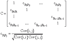
Correlation Matrix |
|
If the standard errors are too high and the confidence intervals are too wide, additional research needs to be done. One cause could be a redundancy in the selected model, meaning that several parameters of the model correlate with one another. Here, the correlation matrix is useful. For completely uncorrelated parameters, you cannot compensate for deterioration of the curve fitting, caused by changing a parameter, by adapting one of the other parameters. You can, however, do this for fully correlated parameters. This also means that the parameters cannot be clearly determined. Example: y = P0P1x |
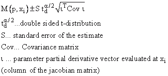
Confidence Band |
|
The output is 95%, 99% and 99.9%. |
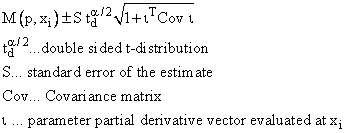
Prediction Band |
|
The output is 95%, 99% and 99.9%. |
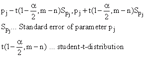
Confidence Intervals of Parameters |
is the 100(1-alpha)% confidence interval for a parameter |
It would not be accurate to state that for a 90% confidence interval, the probability that a parameter lies within the interval is 90%. This would only be the case if you had an infinite number of data points available. In other words, if you repeated the experiment ceaselessly, then 90% of the confidence intervals would contain the respective parameter. The output is 95%, 99% and 99.9%. |
Standard Error of Parameters |
|
|
Goodness-of-Fit
•Convergence criteria for non-linear regression determine:
After each iteration step, the function should be tested for the least square mean error (χ² function). The newly determined parameters will be compared with the best result up to this point. If the newly calculated parameter is better, then this one is saved.
•Examine residual scatter diagram:
The residuals should show random distribution of 0 and no recognizable pattern. If the residuals increase or decrease over time, for instance, then this is a sign that another model would be better or a weighting is required.
•Look at the curve of the regression model:
The data values should lie distributed randomly above and below the curve.
•Check how well the selected model describes the data:
οCheck R2:
R2 = 1.0 means that the curve goes through each data point.
R2 = 0.0 means that the regression model does not describe the data any better than as a horizontal line through the mean value of the data.
•Residual sum of squares:
An ideal curve fitting returns 0 as the result.
•The standard error of the estimator is the standard deviation of the differences between the entered data and the adapted model. This gives you insight into how the residuals are distributed by the mean value. An ideal curve fitting would return the value 0.
•Check whether the calculated values make any sense, for instance, make sure that you have not contradicted any laws of physics.
•Look at the confidence interval.
If the confidence interval is too wide, the curve fitting will not be clear. Other values could lead to a similar result.
•It is possible to find the wrong minimum. This could be the case if it is a local minimum, but would not be the case for a global minimum. Therefore, it is important to find good initial values for the selected model.
Several tests with different initial values increase the probability that the results are correct.
References
•P.R. Bevington, D.K. Robinson. Data Reduction and Error Analysis for the Physical Sciences, 3rd Ed., McGraw-Hill, New York, 2003.
•J. Hartung. Statistik. Lehr- und Handbuch der angewandten Statistik (Textbook and Manual on Applied Statistics). 9th Edition. Oldenbourg Verlag, 1993.
•Harvey Motulsky, Arthur Christopoulos. Fitting Models to Biological Data Using Linear and Nonlinear Regression: A Practical Guide to Curve Fitting. Oxford University Press, 2004.
See Also
Non-Linear Curve Fitting Analysis Object
You might be interested in these articles
You are currently viewing a placeholder content from Facebook. To access the actual content, click the button below. Please note that doing so will share data with third-party providers.
More InformationYou need to load content from reCAPTCHA to submit the form. Please note that doing so will share data with third-party providers.
More InformationYou are currently viewing a placeholder content from Instagram. To access the actual content, click the button below. Please note that doing so will share data with third-party providers.
More InformationYou are currently viewing a placeholder content from X. To access the actual content, click the button below. Please note that doing so will share data with third-party providers.
More Information


